Page 191 - GIS for Science, Volume 3 Preview

Is it safer to ride on bike paths?
The next assignment focused on a well-known challenge: improving bicycle safety. The number of bicycle fatalities has reached a 30-year high in the United States, because of more bicyclists on the road, cars driving at faster speeds, distractions from cell phones, and the lack of bike path infrastructure. The task was to examine whether bicyclists were more likely to be injured if they were on a bike path. The assignment asked the teams to describe severity of injuries depending on several factors, including characteristics of the zip code where the accident occurred, and accident-related factors, such as whether alcohol was involved. Students retrieved bike path and other spatial data layers from the SANDAG, accident information from the Statewide Integrated Traffic Records System at UC Berkeley, and business data from the City of San Diego. Students also generated additional variables through the ArcGIS geoenrichment service.
The likelihood of getting into a collision on a bike path depended on how bike paths were defined in the first place, and how the accident locations were recorded (as either geocoded addresses, or GPS coordinates, or both). In each case, students had to choose more accurate coordinates and define a distance buffer around bike paths so that they could approximately place accidents on a bike path or outside of it. As before, these design choices resulted in different modeling results, often forcing students to reconsider their approach.
Using exploratory analysis,
students found that biking
accidents are more likely to
occur in zip codes where more
alcoholic beverages are sold
and that accidents on bike
paths generally resulted in
fewer severe injuries. Students
chose the data science
algorithms for their analysis.
In most cases, the choices
about how to define spatial
features and compute spatial
relationships for inclusion
in machine learning models had a larger effect on the accuracy of results than a selection of a machine learning technique. That was an important takeaway from this exercise and from the course as a whole.
Suitability modeling
In this next mini-project, students tried to find and organize raster data in ArcGIS Living Atlas of the World, converted from vector data of their choice or published as an ArcGIS raster image collection from scenes downloaded from the US Geological Survey. The raster layers were clipped to a study area and remapped for inclusion in a suitability or a risk model, which students implemented using raster analytics functions in ArcGIS API for Python on the ArcGIS Enterprise installation at UCSD Library. Besides demonstrating the machinery of raster analytics and map algebra functions, this exercise showed that model results differed depending on the map combination techniques used by students, such as exclusionary screening or a weighted linear combination of factors expressed as raster layers.
As with the previous mini-projects, the students were expected to discuss how their choices—such as the raster layers they selected, the remapping rules for each layer, the map algebra and map combination techniques, and the assigned
weights—affected the results. Within these general expectations, topics of student mini-projects ranged from determining suitable locations for soccer fields in San Diego and highlighting wildfire or desertification risks, to finding best sites for rock climbing, mountain biking or camping, locating wildfire alarm outposts and drive- through restaurants. Grading such open-ended assignments is time-consuming but the reward is better student learning as they creatively apply spatial analysis techniques to intriguing problems.
Why spatial is special in machine learning
The key takeaway from this course: knowing how to find, interpret, and efficiently use spatial information through spatial APIs in a common coding environment 1) lets users create more comprehensive datasets by integrating data from different sources, 2) makes data science projects more visually attractive and 3) helps improve performance of machine learning models. One example is more accurate prediction of childhood asthma hospitalization rates—information that would help hospitals better allocate personnel and other resources, and help families with affected children. This class explored a random forest regression and computed asthma hospitalization rates with and without spatial variables, resulting in improved model accuracy using spatial data.
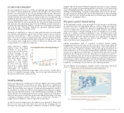
Asthma hospitalization data is sometimes incomplete. Besides asthma hospitalization rates by some (but not all) Connecticut census tracts, additional variables reflect educational attainment, unemployment, other health indicators, and income levels. Using these variables, obtained through geoenrichment, we built a predictive model to impute the missing asthma hospitalization values. Using random forest regression in scikit-learn, we experimented with various model parameters and derived the best model, which gives us a prediction accuracy of 0.73 on the testing set. Then, we can try to predict asthma hospitalization rates, but with additional spatial data layers, such as distance to toxic release points and to primary and secondary roads. Using the Forest-based Classification and Regression tool in ArcGIS.Learn increased the prediction accuracy and allowed the model to be applied to a similarly geoenriched layer at a finer spatial granularity.
The next snapshot shows a fragment of a Jupyter notebook with a map of predicted child hospitalization rates by block groups, as computed by the model.
Teaching Spatial Data Science and Deep Learning 179