Page 154 - GIS for Science, Volume 3 Preview

GIS WORKFLOW FOR SOUNDSCAPE MODELING
Step 5: Repeat
At this point, researchers repeat the acoustic simulation for all sources of noise, including all ships, global wind, and waves. The acoustic intensity from each of these sources is summed with the transmission loss computed using the propagation model to determine how loud the ocean is in every location.
Step 6: Analysis
Using this global ambient noise model can help answer questions related to acoustic communications, marine mammal stressors, and optimal acoustic sensor placement for various oceanographic sensing or defense applications.
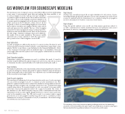
A
The six-step process of a typical ocean acoustic GIS workflow involves synthesizing a vast array of environmental input data and making that data available to an acoustic propagation model, such as a ray trace simulation
or parabolic equation-based model. The workflow then takes
the results of the acoustic simulation and uses analysis tools to answer questions ranging from how far away one bowhead whale can hear another bowhead to where sensors should be placed to detect a vessel fishing illegally in a closed area. This workflow resembles an hourglass, which is wide at both ends and narrow in the middle. The top of the hourglass represents the data management and processing required to feed the acoustic model what it needs. The bottom represents the wide range of analysis techniques that can be applied to the results of the acoustic simulation. The narrow middle represents the acoustic simulation itself. The wide parts— the top and bottom of the hourglass—are both GIS.
Step 1: Gather data
Acoustic propagation is affected by an array of ocean properties. The data for each of these properties (and providers) includes: oean temperature (map A)and ocean salinity (World Ocean Atlas); ocean bathymetry (the General Bathymetric Chart of the Oceans); bottom type (Bottom Sediment Type v 2.0 database); wind and wave height (National Atmospheric and Oceanographic Administration); and ship location (Spire).
Step 2: Dependent variables B Temperature, salinity, and pressure are used to calculate the speed of sound in
seawater (map B). Bathymetry and information about bottom composition are used
to determine how the sound will reflect off of and be absorbed by the seafloor.
Step 3: Grid data
The manner in which the environmental data is discretized and gridded is critical for acoustic modeling. For example, the parabolic equation-based acoustic models used by this team require the acoustic field to be computed every one-half wavelength. A 50 Hz sound has a wavelength of 30 m.
Step 4: Acoustic simulation
The sound speed, bathymetry, bottom characteristics, and source location are input into an acoustic propagation model to estimate acoustic transmission loss. This parabolic equation-based model conducts the simulation along radials at discrete bearings and then integrates the resulting vertical slices into a full 3D field using s patial interpolation. Horizontal refraction is also accounted for because subtle horizontal sound speed gradients deflect the sound horizontally. The result of the simulation is the channel impulse response (CIR), a mathematical term that represents how the acoustic signal changes between a source location and every voxel in the simulation area. The CIR can be used to reconstruct what a signal generated in one location might sound like in another location, or estimate acoustic transmission loss (map C). Transmission loss (TL) is a measure of how much energy is lost between source and receiver.
C
142
GIS for Science
The complexity of the ocean acoustics modeling challenge results from the data being volumetric. In the GIS workflow, the water “layers” are combined in a model to create layers that can describe the long-distance behavior of sound in the world’s oceans.