Page 28 - GIS for Science, Volume 3 Preview

10 1-km segments comprising the 10-km coastline length. For subsequent classification and description purposes, we identified three sinuosity classes (straight, sinuous, and very sinuous) based on ranges of the RI (Table 8).
9. Slope profile
“transferred” to corresponding locations on the GSV. MERIT Hydro rivers are associated with basin delineations, and these basin areas were used to approximate the average annual discharge for the rivers.
Using the WorldClim version 2.0 data,46 the long-term (30 years) average annual precipi- tation figures for all 1-km cells containing river mouth locations were obtained. This river mouth precipitation value was treated as a uniform measure of the quantity of water falling in every cell in the basin, acknowledging that in reality there will be some level of spatial variation in precipitation input across the watershed. The precipitation quantity at the river mouth was multiplied by the total number of cells in the basin as an approxima- tion of the average annual total amount of water falling in the watershed. This total wa- tershed input quantity was used as a proxy for the discharge amount at the river mouth location in a “what pours in must spill out” sense, acknowledging that some of the input precipitation will be evapotranspirated or lost to groundwater flow and therefore will not arrive at the river mouth. The river discharge was then spatially distributed from the river mouth into the ocean using a statistical smoothing (kernel density) operation to identify a normalized spatial footprint and magnitude of river outflow.
When freshwater discharges into estuaries and the ocean, the spatial dynamics of the mixing waters are complex.61 Plumes form in the mixing zone based on properties of the freshwater inputs (quantity, velocity, composition, etc.) and the receiving ocean environment (currents, tides, waves, obstructions, etc.).59 Differences in the magnitude of freshwater influence in the coastal zone from one river to the next could indeed be assessed from a robust characterization of plume dynamics, but the spatial and tem- poral characterization of riverine discharge plumes globally is currently impractical and well beyond the scope of this exercise.
The team instead developed a standardized, spatial measure of freshwater “influence” using a quartic statistical kernel density algorithm62 that spread the river discharge into the ocean as a probability smoothing function. This measure, which we call a river out- flow index, describes the relative spatial distribution and magnitude of the riverine in- put and is in essence a potential spatial footprint of river influence in the coastal zone. Importantly, the spatial distribution and magnitude of the modeled river outflow is not intended to represent actual plume shapes and sizes; rather, it is a conceptual geospa- tial model of the relative influences of fluvial processes in the coastal zone. Essentially, we have modeled a standardized, potential river discharge footprint in the absence
of currents or other directional energies or non-coastal barriers. This variable captures spatial differences in river outflows as a simple measure of land-to-sea influence.
A 1-km raster framework was established for the purpose of calculating a river outflow index for each segment using a moving neighborhood analysis window (NAW), such
as is commonly used in DEM processing for calculations of terrain attributes. The
NAW size was 1 decimal degree (~ 110 km). The spreading function was constrained seaward to a distance of approximately 55 km, the seaward limit of the NAW. Land- ward, the shoreline vector acted as a hard boundary preventing the spreading function from allowing the backward flow of water onto the land. The river outflow index data are continuous data in a 1-km raster grid and represent a NAW-derived measure of
the magnitude (expressed as the spatial distribution) of the amount of precipitation/ riverine discharge that has been spread from the cell. Specifically, the river outflow index characterizes the size (expected number of pixels) of the spatial footprint created by the spread of discharge into the ocean. The coastline segment midpoints were at- tributed with the river outflow index value from the raster cell whose center was closest to the segment midpoint. For subsequent classification and description purposes, the river outflow index values were rescaled from zero to one using a minimum-maximum method and grouped into three levels (low, moderate, and high) of fluvial importance (Table 10).
Coastal areas can contain steeply sloping
mountains plunging into the ocean, low
gradient mudflats with almost impercepti-
ble sloping in a seaward direction, and ev-
erything in between. Slope is a determinant
of the width of the littoral zone, which can
range from narrow steep beaches to wide
tidal flats.53 The slope gradient at the coast-
line influences many aspects of wave energy
and shoaling, swash zone morphodynamics,
sediment deposition and erosion,54 and associated differences in biotic distributions.55 Slope gradient is a strong determinant of changing coastline position and is particularly important in the analysis of shoreline retreat from sea-level rise.56 Interest in assessing change in coastline position has led to the development of methods (e.g. Doran et al.57) for calculating coastal slope gradient.
Our team developed a global coastline slope profile datalayer by extending a perpen- dicular line from each segment midpoint 100-m in landward and seaward directions. The endpoints of this 200-m vector were attributed with elevation values from the corre- sponding raster cells that contained the 200-m perpindiculars. The elevation data source was the 15 arc seconds (~500-m) resolution GEBCO (General Bathymetric Chart of the Oceans) bathymetry and topography resource,58 sharpened and gap-filled using data from an Airbus® global 12-m spatial resolution DEM. The slope values of the 200-m segments were attributed as continuous data to the segment midpoints. For subse- quent classification and description purposes, we grouped the slope values into four categories: (flat, sloping, steeply sloping, and vertical (Table 9) based on CMECS classes and value ranges.
10. River outflow index
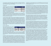
Slope Class
Slope Range (%)
Flat
Less than 8.75
Sloping
8.75–57.3
Steeply Sloping
57.3–173.2
Vertical
More than 173.2
Rivers and streams are the source of fresh-
water inputs and particulate matter to the
coastal zone, structuring important ecosys-
tems such as estuaries and deltas. Sediment
discharge at the mouth of rivers along the
coast is the source of most sediment in the
coastal zone,8 and river outflow influences
coastal zone dilution processes, nutrient
levels, sediment and particulate organic matter composition, pollutant and pathogen exposure levels, etc.59 River-dominated systems are one of three fundamental deposi- tional morphotypes in coastal areas, along with tide-dominated and wave-dominated systems.17,18
Using data from approximately 160,000 rivers, we developed a global coastal river out- flow index to capture the global distribution and magnitude of annual discharge of rivers at the coastline. The river outflow index was the most complex of the 10 ecological set- tings variables attributed to the coastline segments. Unlike the other nine variables, all of which represent physical measurements of the coastal environment, the river outflow index is a modeled value of the magnitude and extent of riverine influence. We first ob- tained global river mouth data from the MERIT (Multi-Error-Removed Improved Terrain) Hydro resource.60 MERIT Hydro rivers are interpreted from a hydrologically conditioned 3 arc second (~ 90-m) global digital elevation model (DEM), and, unless they drain in- ternally in an inland basin, terminate at a river mouth where the land meets the ocean. River mouth locations were obtained from the MERIT Hydro resource and subsequently
Table 9
Fluvial Importance
River Outflow Index (unitless)
Low
0–.000012
Moderate
.000013–.001128
High
.001129–1.0
16
GIS for Science
Table 10